
Gram-Schmidt Orthonormal Model
Published:
This blog explores a semi-supervised approach to binary classification for topic modeling. The primary advantage of this approach is the reduced need for large labeled datasets, addressing a key limitation in supervised learning for natural language processing (NLP): achieving strong performance with minimal labeled data.
A state-of-the-art semi-supervised method for binary classification.
Author: Ahmad Rammal
Introduction
Binary classification in NLP is traditionally approached using supervised learning. In this framework, models learn to map new examples by analyzing labeled training data. However, supervised methods require substantial labeled datasets, which are costly and time-consuming to create. This is particularly challenging in NLP, where human annotators are often needed to produce high-quality labels.
Semi-supervised learning offers a compelling alternative. By leveraging both labeled and unlabeled data, semi-supervised methods significantly reduce the dependence on extensive labeled datasets. Furthermore, these models decouple the embedding generation process from classification, enabling efficient reuse of embeddings for other NLP tasks.
Model Overview
I. Mean Model
Concept
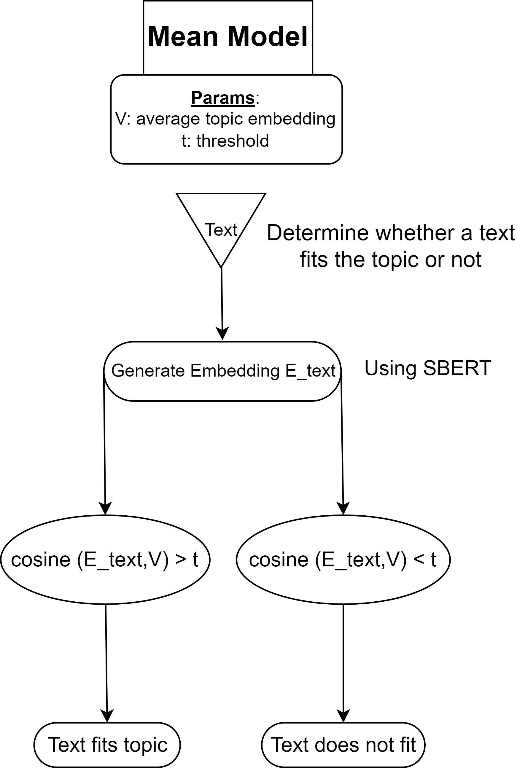
The Mean Model classifies text as fitting (1) or not fitting (0) a given topic based on cosine similarity. The process begins by generating a vector representation of the text (embedding) using a sentence embedding model like SBERT. Let this vector be $E_{\text{text}}$.
The topic is also represented as a vector $V$, derived from its keywords. The cosine similarity between $E_{\text{text}}$ and $V$ determines the semantic closeness of the text to the topic. A threshold $t$ is defined such that:
If $\cos(E_{\text{text}}, V) > t$, the text is classified as fitting the topic. Otherwise, it does not.
Training
Training involves two key steps:
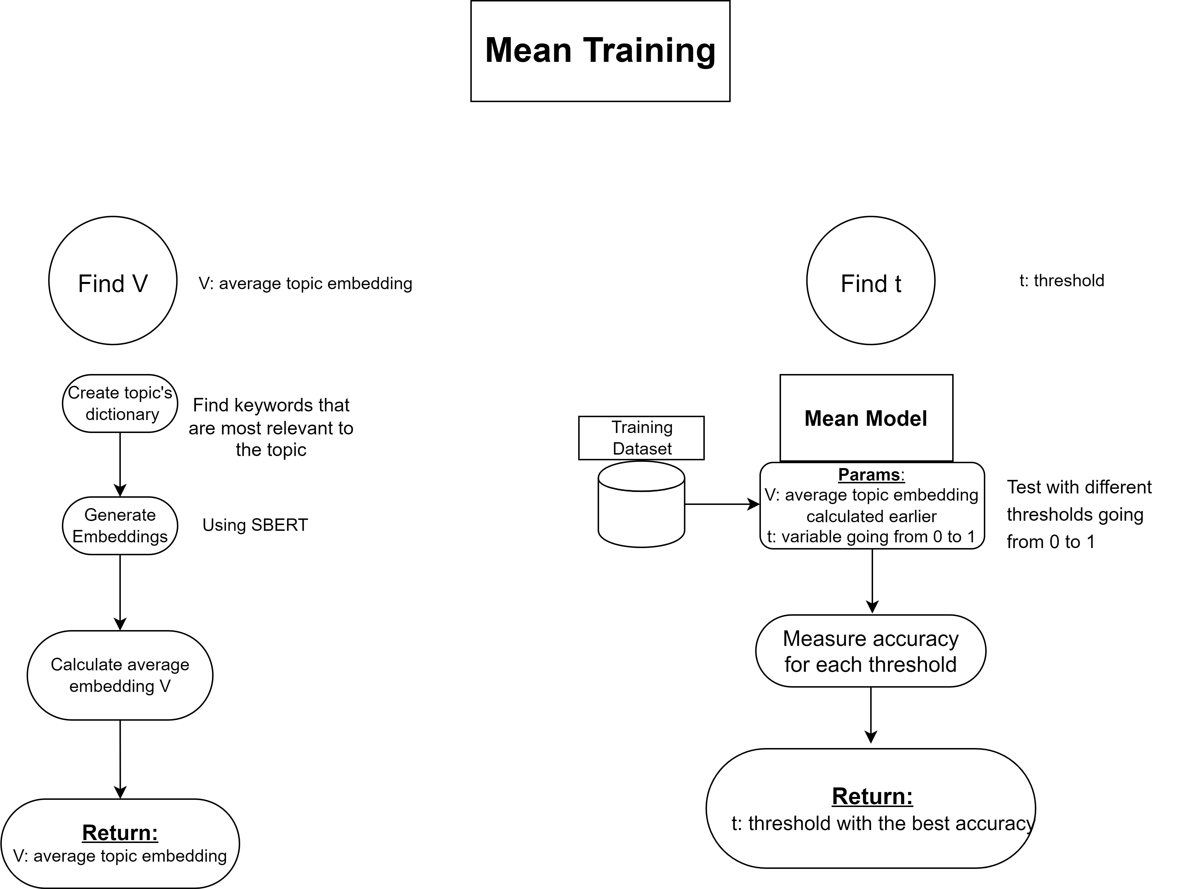
Defining the Topic Vector $V$:
Keywords relevant to the topic are identified manually to form a dictionary. Embeddings for these keywords are generated, and their average yields the topic vector $V$.Determining the Threshold $t$:
The model is tested on a labeled dataset with thresholds ranging from 0 to 1. The threshold providing the best accuracy is selected.
II. Gram-Schmidt Model
Concept
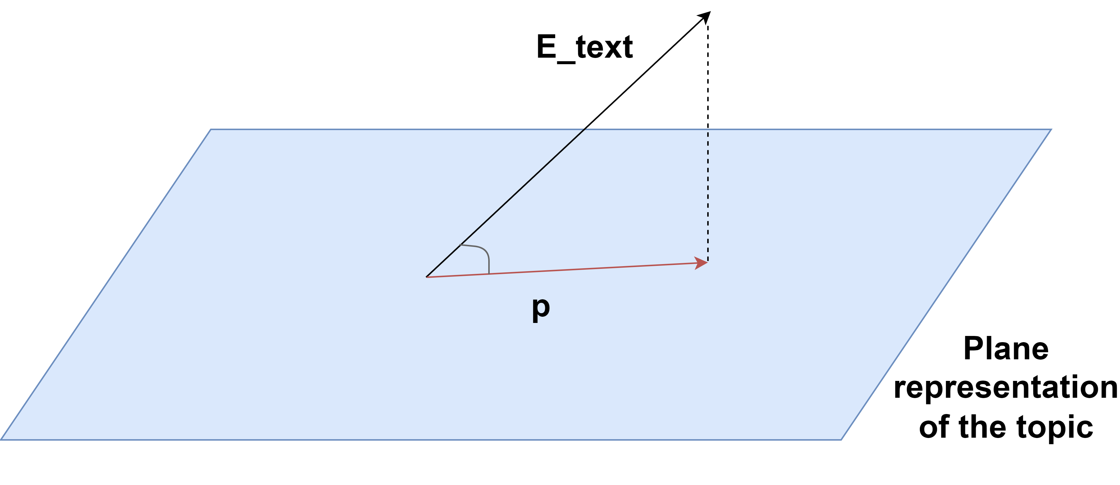
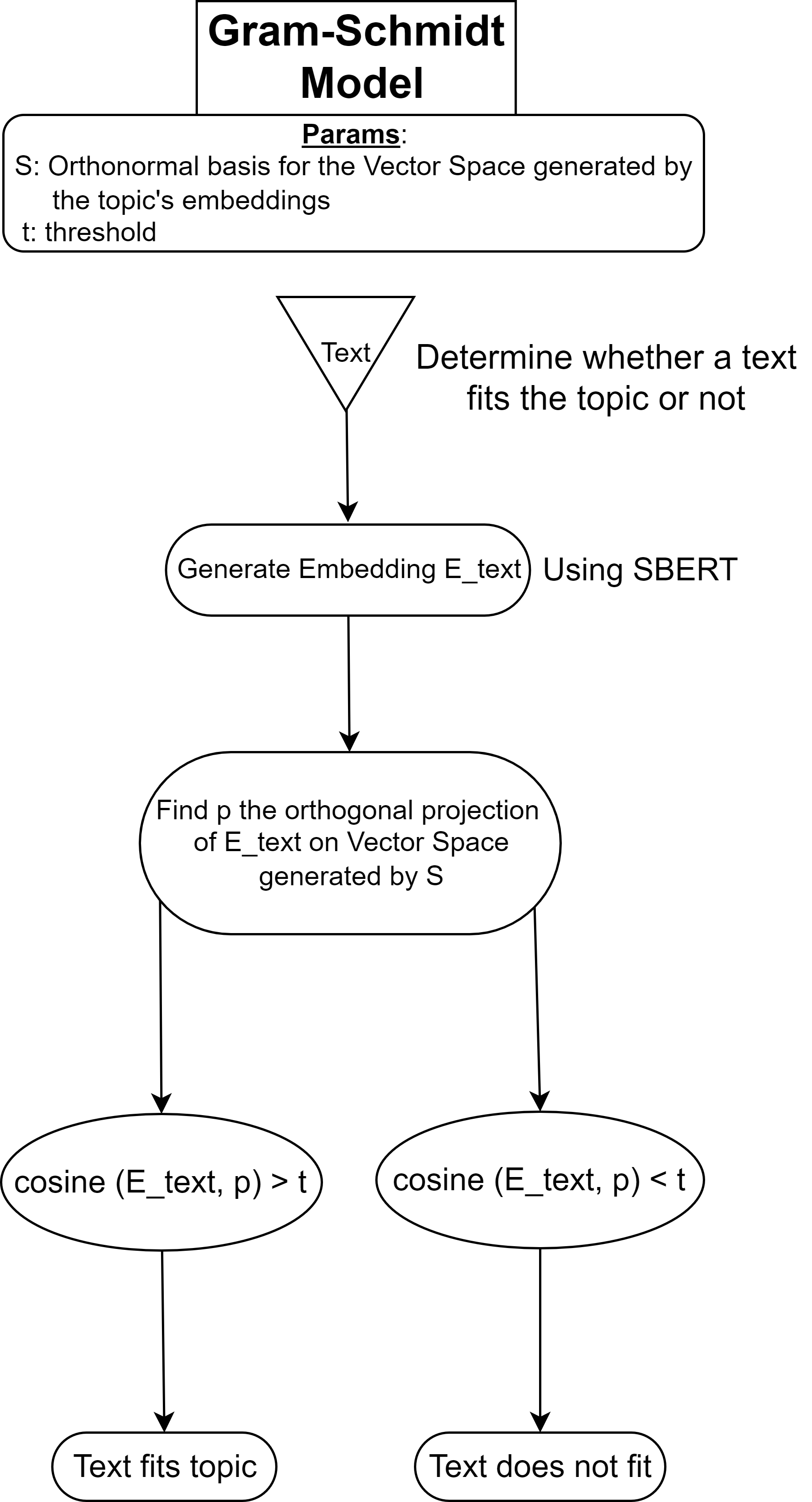
Building upon the Mean Model, the Gram-Schmidt Model represents a topic as a vector space instead of a single vector. This space is defined by an orthonormal basis generated using the Gram-Schmidt process.
For a given text, its vector representation $E_{\text{text}}$ is orthogonally projected onto the topic vector space. The cosine similarity between $E_{\text{text}}$ and its projection $p$ quantifies the semantic closeness of the text to the topic.
As in the Mean Model, a threshold $t$ is used to classify the text.
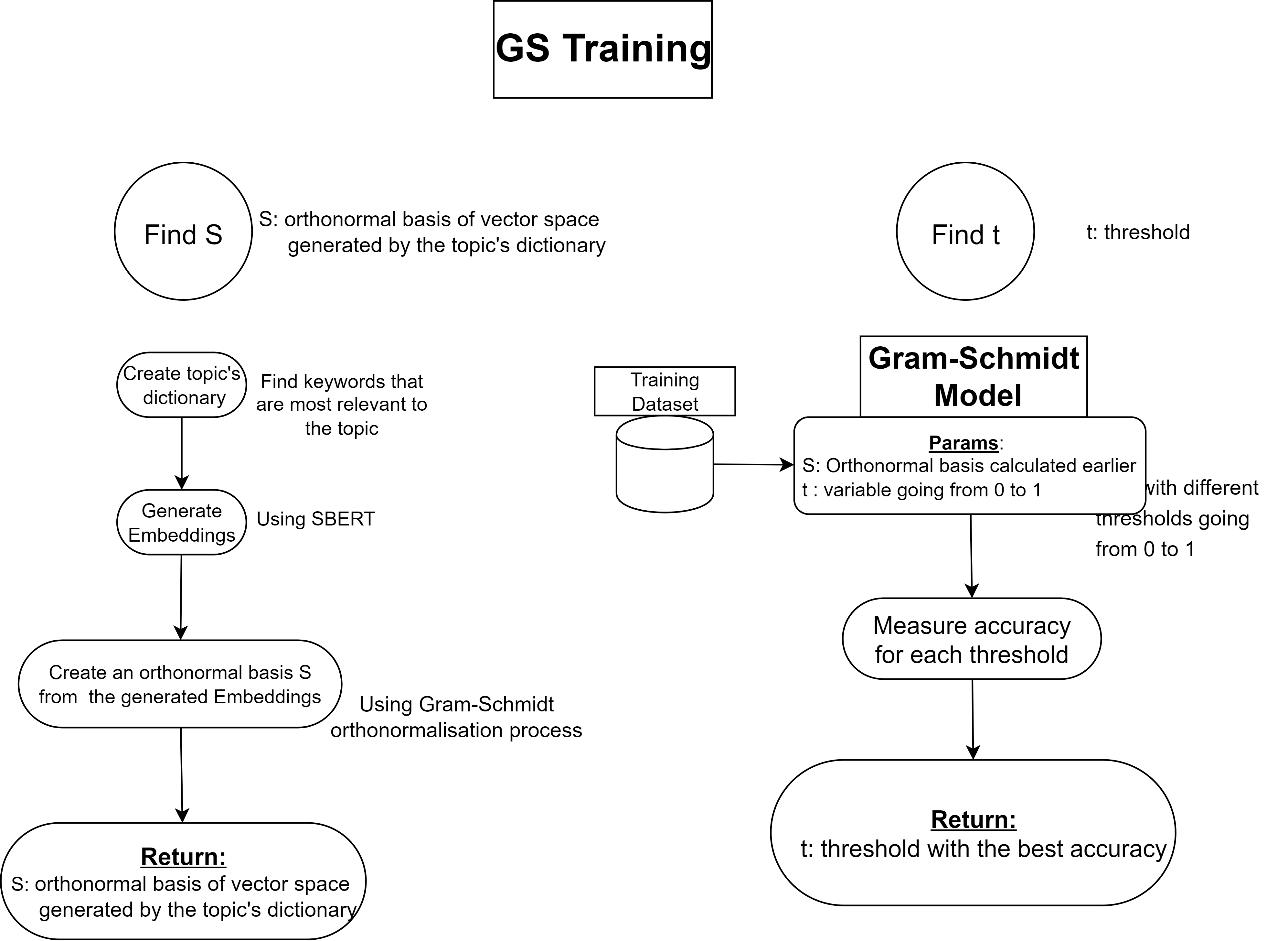
Training
Creating the Orthonormal Basis $S$:
Relevant keywords are manually selected, and their embeddings generate the topic’s vector space. The Gram-Schmidt process is then applied to produce an orthonormal basis.Determining the Threshold $t$:
Similar to the Mean Model, the threshold is selected based on performance on a labeled dataset.
Advantages of the Approach
This semi-supervised structure relies solely on generic models like SBERT, eliminating the need for fine-tuning. By decoupling embedding creation from classification, embeddings can be reused for tasks like clustering or different classification problems, saving significant computational resources.
Performance Evaluation
Metrics for an environmental classification task are summarized below:
| Metric | FinBERT | Mean | Gram-Schmidt (GS) |
|---|---|---|---|
| Accuracy | 0.903 | 0.849 | 0.926 |
| Precision | 0.924 | 0.832 | 0.939 |
| Recall | 0.877 | 0.873 | 0.910 |
| F1-Score | 0.900 | 0.852 | 0.924 |
The Gram-Schmidt Model outperforms FinBERT, with the Mean Model achieving respectable results. These findings demonstrate the efficacy of semi-supervised methods as a viable alternative to traditional supervised approaches.